A Simple Excel VBA Code Example
In this example, we want to track expenses and calculate the day totals as well as each category total. We will see how these calculations are achieved manually in ten steps and create a button to perform these in one click.
1. Open a new Excel workbook.
2. Go to the Tools menu; choose Macro, and then Record New Macro… Type Expenses in the Name field and press OK.
3. Go to cell B1 and type Food.
4. Go to cell C1 and type Gas.
5. Go to cell D1 and type Other.
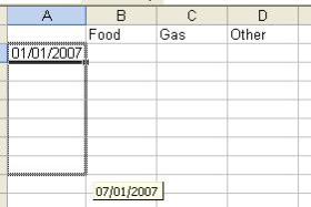
6. Go to cell A2 and type 01/01/07.
7. When a cell is selected there is a small square at the bottom right side of the selection rectangle. As you place the mouse over the small square, the cursor will change from a wide white plus sign to a thin black plus sign. Press the left mouse button on thin black plus sign and slowly drag it down to cell A8. As you drag the plus sign downward the consecutive dates form 02/10/07 to 07/01/07 will appear to the right of the plus sign. Excel will automatically fill in the corresponding cells with these value when you release the mouse button.
8. While 07/01/07 is showing, release the mouse button.

9. Press the Stop Recording button. If you closed the very small window with the Stop Recording button, go to Tools, Macro, Stop Recording.
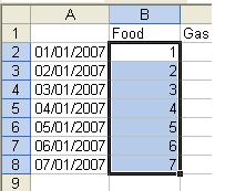
10. For the sake of simplicity, fill in the cells under Food with the values 1-7.
11. Select the cells B2 through B8 by dragging the mouse over them:

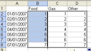
12. Drag the small black rectangle
at the bottom of the selection to the right until you see that the
selection includes the D column and release the mouse button:

In this Excel VBA code example we want to see the sums of the expenses for both the days and the categories.
13. Turn on the recorder again. Tools > Macro> Record New Macro… Type Sums in the Name field and press OK.
14. Choose the cell E2 and press the sigma sign on the toolbar and press Enter:

15. Choose the E2 cell again and
drag the small rectangle at the bottom-right down to cell E8.


15. Release the mouse button:


16. Choose the cell B9 and press
the sigma sign on the toolbar and press Enter
17. Choose the B9 cell again and drag the small rectangle at the bottom-right down to cell E9.
18. Press the Stop Recording button or go to Tools, Macro, Stop Recording.
Now it’s time to examine and customize our Excel VBA code example. We will customize it so that it will work not only when there are 7 day rows, but also with however many days/rows we add.
Hold down one of the ALT keys next to the spacebar and press
F11 to go to the Visual Basic Editor, and then release the ALT
key. The following is basically what you should see:
Sub Expenses()
Range("B1").Select
ActiveCell.FormulaR1C1 = "Food"
Range("C1").Select
ActiveCell.FormulaR1C1 = "Gas"
Range("D1").Select
ActiveCell.FormulaR1C1 = "Other"
Range("A2").Select
ActiveCell.FormulaR1C1 = "1/1/2007"
Range("A2").Select
Selection.AutoFill Destination:=Range("A2:A8"), Type:=xlFillDefault
Range("A2:A8").Select
End Sub
Sub Sums()
Range("E2").Select
ActiveCell.FormulaR1C1 = "=SUM(RC[-3]:RC[-1])"
Range("E2").Select
Selection.AutoFill Destination:=Range("E2:E9"),
Type:=xlFillDefault
Range("E2:E9").Select
Range("B9").Select
ActiveCell.FormulaR1C1 = "=SUM(R[-7]C:R[-1]C)"
Range("B9").Select
Selection.AutoFill Destination:=Range("B9:E9"),
Type:=xlFillDefault
Range("B9:E9").Select
End Sub
If for some reason you don’t see this code, notice the
VBAProject title bar below the toolbar icons at the upper left of the screen. If you have only one workbook open, and you should, you will see a tree view of the Microsoft Excel Objects and Modules. They appear as yellow folders. Click on the + to open the branches. Double click on the last Module under Modules
and the code should be there. If you’ve never worked with the
Excel VBA Editor before, there should only be one Module under
Modules.
As we saw with the Macro Recorder in Word, here too it
types/creates code in a deliberate manner. As you can probably
guess by now, Range("B1").Select was our selecting the cell B1
and ActiveCell.FormulaR1C1 = "Food" was our typing in the
word, called a Value, "Food."
If we were manually typing this, we could have coded the same end result as, Range("B1").Value = "Food". So again, at this point you shouldn’t be overly concerned about or trying to memorize the code that we are creating with the recorder.
To keep our Excel VBA code example simple, let’s not go into
the code that the recorder recorded. Excel created it and it will always work for us. What we want to learn is how to adapt or customize this code to work independent of there being
exactly 7 rows or days…
To do this we will have use strings and manipulate them. String
are any text, which by definition are any letters, numbers, and/or symbols surrounded by quotes, i.e. "VBA," that the parent
application won’t try to understand as being Keywords, or words
that have specific meanings in VBA.
There are two things we will have to accomplish for our code to
be able to handle a variable amount of rows/days…
The first is that we have to find out how many rows are in the
workbook that we would be currently running the code in. And
second, change two lines of code that presently are set up to to
assume that there are 7 rows with dates, or 7 days.
To help us with the first, I’ll record a quick macro. You can save time and not do this. I turned on the recorder and pressed Ctrl + End, holding down one of either of the two Ctrl keys and then pressing the End key, and then releasing the Ctrl key. After stopping the recorder, this was what Excel typed for the code that we’ll use:
ActiveCell.SpecialCells(xlLastCell).Select
It says "Select the last used cell."
There is one problem that could arise from using this statement
or command. If we wanted to track expenses for say 14 days, we
would drag the small rectangle down from the first date until we
saw the 14th date, say 14/01/07. If we were to drag it by accident to 16/01/07 and then delete the 15th and the 16th, Excel would consider the last used cell to be in the row where the 16th was. We’ll overlook this in this example.
After this line will run, as we’ve said, the Active or Selected cell will be what Excel has determined to be the last cell on the active spreadsheet. We can now use a variable, or "place holder," to hold on to the row number of the last row. Like this:
LastRow = ActiveCell.Row
Now, we have to get this value, which is 9 in our case but could
be a different last row in another, into the the following two
statements:
ActiveCell.FormulaR1C1 = "=SUM(R[-7]C:R[-1]C)"
and
Selection.AutoFill Destination:=Range("B9:E9"), Type:=xlFillDefault
In the first, we can see that LastRow will have to be adjusted and inserted in place of the 7, which represents the 7 rows of dates. We know that in our example, LastRow, which is 9, would need to be adjusted to 7. the difference of 2 is because the first row contains the headers Food, Gas, and Other, and the actual sum will be in the row after the 7 date rows. If there were 14 dates the sum would be in row 16, etc.
LastRow = LastRow - 2
LastRow now holds the value of 2 less than the value of what LastRow was.
Our new sub procedure Sub Sums() will now look like this:
Sub Sums()
Range("E2").Select
ActiveCell.FormulaR1C1 = "=SUM(RC[-3]:RC[-1])"
Range("E2").Select
Selection.AutoFill Destination:=Range("E2:E9"), Type:=xlFillDefault
Range("E2:E9").Select
Range("B9").Select
LastRow = LastRow - 2
' Remember, a line that starts with an apostrophe is a comment line
' I’m leaving the lines we are replacing here for reference
' ActiveCell.FormulaR1C1 = "=SUM(R[-7]C:R[-1]C)"
ActiveCell.FormulaR1C1 = "=SUM(R[-" & LastRow & "]C:R[-1]C)"
' Range("B9").Select
Range("B" & LastRow).Select
' Selection.AutoFill Destination:=Range("B9:E9"), Type:=xlFillDefault
Selection.AutoFill Destination:=Range("B" & LastRow & ":E" & LastRow), & _
Type:=xlFillDefault
' Range("B9:E9").Select
' We actually don’t need this last row of code since
' we don’t need the last cell to be active/selected.
End Sub
Another Simple Excel VBA code example.
Using the VBA Label to Create Flash Cards.
In this Excel VBA code example create flash cards in Excel.
Finding the Last Populated Cell, Row, or Column in a Worksheet
An Excel VBA code example showing how to find the last populated.
How to cause code to be run when Excel opens
A simple Excel VBA code example showing how to make your code run when Excel opens.
How to move to cell
Learn how to move to a specific cell, such as the maximun value in a Worksheet, in this Excel VBA code example
How to delete column
An Excel VBA code example showing how to delete a column.
17. Choose the B9 cell again and drag the small rectangle at the bottom-right down to cell E9.
18. Press the Stop Recording button or go to Tools, Macro, Stop Recording.
Now it’s time to examine and customize our Excel VBA code example. We will customize it so that it will work not only when there are 7 day rows, but also with however many days/rows we add.
Hold down one of the ALT keys next to the spacebar and press
F11 to go to the Visual Basic Editor, and then release the ALT
key. The following is basically what you should see:
Sub Expenses()
Range("B1").Select
ActiveCell.FormulaR1C1 = "Food"
Range("C1").Select
ActiveCell.FormulaR1C1 = "Gas"
Range("D1").Select
ActiveCell.FormulaR1C1 = "Other"
Range("A2").Select
ActiveCell.FormulaR1C1 = "1/1/2007"
Range("A2").Select
Selection.AutoFill Destination:=Range("A2:A8"), Type:=xlFillDefault
Range("A2:A8").Select
End Sub
Sub Sums()
Range("E2").Select
ActiveCell.FormulaR1C1 = "=SUM(RC[-3]:RC[-1])"
Range("E2").Select
Selection.AutoFill Destination:=Range("E2:E9"),
Type:=xlFillDefault
Range("E2:E9").Select
Range("B9").Select
ActiveCell.FormulaR1C1 = "=SUM(R[-7]C:R[-1]C)"
Range("B9").Select
Selection.AutoFill Destination:=Range("B9:E9"),
Type:=xlFillDefault
Range("B9:E9").Select
End Sub
If for some reason you don’t see this code, notice the
VBAProject title bar below the toolbar icons at the upper left of the screen. If you have only one workbook open, and you should, you will see a tree view of the Microsoft Excel Objects and Modules. They appear as yellow folders. Click on the + to open the branches. Double click on the last Module under Modules
and the code should be there. If you’ve never worked with the
Excel VBA Editor before, there should only be one Module under
Modules.
As we saw with the Macro Recorder in Word, here too it
types/creates code in a deliberate manner. As you can probably
guess by now, Range("B1").Select was our selecting the cell B1
and ActiveCell.FormulaR1C1 = "Food" was our typing in the
word, called a Value, "Food."
If we were manually typing this, we could have coded the same end result as, Range("B1").Value = "Food". So again, at this point you shouldn’t be overly concerned about or trying to memorize the code that we are creating with the recorder.
To keep our Excel VBA code example simple, let’s not go into
the code that the recorder recorded. Excel created it and it will always work for us. What we want to learn is how to adapt or customize this code to work independent of there being
exactly 7 rows or days…
To do this we will have use strings and manipulate them. String
are any text, which by definition are any letters, numbers, and/or symbols surrounded by quotes, i.e. "VBA," that the parent
application won’t try to understand as being Keywords, or words
that have specific meanings in VBA.
There are two things we will have to accomplish for our code to
be able to handle a variable amount of rows/days…
The first is that we have to find out how many rows are in the
workbook that we would be currently running the code in. And
second, change two lines of code that presently are set up to to
assume that there are 7 rows with dates, or 7 days.
To help us with the first, I’ll record a quick macro. You can save time and not do this. I turned on the recorder and pressed Ctrl + End, holding down one of either of the two Ctrl keys and then pressing the End key, and then releasing the Ctrl key. After stopping the recorder, this was what Excel typed for the code that we’ll use:
ActiveCell.SpecialCells(xlLastCell).Select
It says "Select the last used cell."
There is one problem that could arise from using this statement
or command. If we wanted to track expenses for say 14 days, we
would drag the small rectangle down from the first date until we
saw the 14th date, say 14/01/07. If we were to drag it by accident to 16/01/07 and then delete the 15th and the 16th, Excel would consider the last used cell to be in the row where the 16th was. We’ll overlook this in this example.
After this line will run, as we’ve said, the Active or Selected cell will be what Excel has determined to be the last cell on the active spreadsheet. We can now use a variable, or "place holder," to hold on to the row number of the last row. Like this:
LastRow = ActiveCell.Row
Now, we have to get this value, which is 9 in our case but could
be a different last row in another, into the the following two
statements:
ActiveCell.FormulaR1C1 = "=SUM(R[-7]C:R[-1]C)"
and
Selection.AutoFill Destination:=Range("B9:E9"), Type:=xlFillDefault
In the first, we can see that LastRow will have to be adjusted and inserted in place of the 7, which represents the 7 rows of dates. We know that in our example, LastRow, which is 9, would need to be adjusted to 7. the difference of 2 is because the first row contains the headers Food, Gas, and Other, and the actual sum will be in the row after the 7 date rows. If there were 14 dates the sum would be in row 16, etc.
LastRow = LastRow - 2
LastRow now holds the value of 2 less than the value of what LastRow was.
Our new sub procedure Sub Sums() will now look like this:
Sub Sums()
Range("E2").Select
ActiveCell.FormulaR1C1 = "=SUM(RC[-3]:RC[-1])"
Range("E2").Select
Selection.AutoFill Destination:=Range("E2:E9"), Type:=xlFillDefault
Range("E2:E9").Select
Range("B9").Select
LastRow = LastRow - 2
' Remember, a line that starts with an apostrophe is a comment line
' I’m leaving the lines we are replacing here for reference
' ActiveCell.FormulaR1C1 = "=SUM(R[-7]C:R[-1]C)"
ActiveCell.FormulaR1C1 = "=SUM(R[-" & LastRow & "]C:R[-1]C)"
' Range("B9").Select
Range("B" & LastRow).Select
' Selection.AutoFill Destination:=Range("B9:E9"), Type:=xlFillDefault
Selection.AutoFill Destination:=Range("B" & LastRow & ":E" & LastRow), & _
Type:=xlFillDefault
' Range("B9:E9").Select
' We actually don’t need this last row of code since
' we don’t need the last cell to be active/selected.
End Sub
More Excel VBA code examples
A Simple Excel VBA ExampleAnother Simple Excel VBA code example.
Using the VBA Label to Create Flash Cards.
In this Excel VBA code example create flash cards in Excel.
Finding the Last Populated Cell, Row, or Column in a Worksheet
An Excel VBA code example showing how to find the last populated.
How to cause code to be run when Excel opens
A simple Excel VBA code example showing how to make your code run when Excel opens.
How to move to cell
Learn how to move to a specific cell, such as the maximun value in a Worksheet, in this Excel VBA code example
How to delete column
An Excel VBA code example showing how to delete a column.
The Excel Worksheets add method
Learn how to move to add a Worksheet in this Excel VBA code example.
Go to the next tutorial: Another Excel VBA Example
Return from An Excel VBA Code Example to VBA Code Samples
